

The CBS production network
The CBS production network for 201810 improves on the 2012 version by integrating more auxiliary micro and industry-level data. Before going into detail it is helpful to explain which are the industry classifications and product classifications used by Statistics Netherlands. Industries are classified using the Dutch Standard Industrial Classifications, in brief SBI, which are equivalent to the European Standard Classification NACE rev.2 in the first two digits, although the subsequent digits can differ. Statistics Netherlands has industry data on two different levels, the SBI4 level, containing 132 industries, and the SBI5 level, corresponding to 888 industries. Regarding the CPA product classification, Statistics Netherlands uses a modified version of the original European CPA, mainly at 4 and 6 digits. In the data, we retrieved 192 commodities for 4 digits and 623 commodities at the 6-digit level.
Firm-level data is obtained from the Statistical Business Register (SBR) for 2018 for over 1, 700, 000 firms. The SBR contains values about net turnover, geographical location, business id, and business sector at the SBI5 classification level. After cleaning for micro-firms with annual net turnover below 10, 000 €, around 900, 000 firms remain, accounting for \(99.5\%\) of the Dutch economy output in 2018. Details regarding the breakdown of output and input at the commodity level are primarily available at the industry level and for a limited number of firms. The Dutch National Supply-Use tables provide data on inter-industry and intra-industry intermediate input/output transactions for various commodities, classified at the Dutch CPA 4-digit level with industries categorized according to the SBI4 level.
While industry-wide transactions are validated, estimating output and input for individual firms per commodity and matching suppliers with users within commodity layers remains a challenge. To estimate supply per firm, domestic turnover, calculated as VAT turnover minus export turnover, is employed as a distributional key. Firms are assumed to supply in proportion to the ratio of their domestic turnover to the overall industry turnover. Additional adjustments are made for wholesale and retail trade firms to account only for domestic turnover associated with actual production.
Estimating use per firm from VAT turnover data involves determining the ratio between intermediate use and turnover. This ratio is estimated using SBS survey data. The breakdown of supply/use per firm at the commodity level is available for a relatively large number of firms through surveys conducted by structural business statistics (SBS) for commercial firms, Prodcom for manufacturing firms, and estimates generated by National Accounts for non-commercial firms.
Specifically, SBS provides a breakdown of sales and intermediate purchases into ten to twenty commodity categories for small firms and at the CPA-classification level for large firms. Prodcom conducts a similar survey. SBS categories are then mapped into CPA commodities by National Account experts.
For firms not covered by the aforementioned surveys, the breakdown in commodities of intermediate supply/use is estimated using the distribution of the industries as a whole from the supply-use tables. This approximation can result in implausible values of annual supply and use. To address this issue, thresholds are imposed, setting supply values below 2000 € and also use values below 1000 € to zero. Finally, an iterative proportional fitting (IPF) procedure is implemented to ensure consistency with industry-level Tables.
Once supply and use per firm per commodity are obtained, their out-degree distribution is estimated using stylized facts from Japanese firms39, connecting out-degrees with firm sizes through a power-law function, while their in-degree distribution is estimated assuming a power-law connection to firm-specific input at the commodity-level, an assumption that is consistent with recent studies on Dutch inter-firm payments26.
Once in-degree and out-degree distributions per commodity are estimated for each firm, suppliers and users are matched according to a deterministic procedure that takes into account (1) a company score, encoding their net turnover, (2) a distance score, that takes into account their mutual distance, (3) the presence of a link between respective industries in the supply-use tables, (4) the presence of the observed relationship in the Dun and Bradstreet dataset, i.e. a dataset containing the list of the users of the 500 largest suppliers in the Dutch Economy. After the computation of the related ‘link score’, users in each commodity layer are ordered according to their purchase volumes. The top user, then, selects the best X suppliers and establish a connection with them, where X represents its commodity-specific in-degree. The procedure continues from the second-highest purchasing volume user to the last until no available links remain and degree distributions are reproduced. Network weights are then distributed across generated links according to a power-law distribution. Finally, the resulting weighted inter-firm network at the 650 commodity level (National CPA level 6) is compared to the Supply-Use tables (National CPA level 4) and consequent adjustments are made to weights and links. Further details can be found in10.
We aggregate the inter-firm network at the commodity level, passing from 623 commodities (CPA level 6) to 192 commodities (CPA level 4, compatible with supply-use tables). Then, we aggregate firms in industries at the SBI5 level, taking their business sector ids from the SBR. For the topic of interest, the self-loops implied by intra-industry trade are not important and can be removed from the dataset without adversely affecting the subsequent analysis. After cleaning for intra-industry trade, we obtain a multi-layer inter-industry production network containing linkages and weights for 862 industries (nodes) and 187 commodity groups (layers).
The firm-level reconstructed dataset is not without limitations. One source of error arises from the breakdown provided by SBS and Prodcom surveys, particularly regarding the documented intermediate purchases and sales. The purchases may include imports, and the sales may also include sales for final consumptive use. Another source of error stems from the distributions and assumptions made for firm out-degree and in-degree distributions. While these assumptions are supported by stylized facts from Japanese firms (for out-degrees) and payment data from a large sample of Dutch firms (for in-degrees), it cannot be assumed that the parameters used in the reconstruction are universally applicable or representative of ‘true values’. Finally, the matching procedure results in a deterministic network where the ‘best’ users have priority in connecting with their more closely aligned suppliers. This algorithm cannot account for noisy behavior or real-world uncertainties. In fact, for the 2012 version, with similar assumptions on degree distributions and the same matching algorithm, it has been demonstrated that these assumptions lead to biases in core network statistics such as the number of links in commodity layers37, when compared with the ground-truth provided by a known sample of firm-to-firm connections collected by Dun and Bradstreet (for 2012). While aggregation at the SBI5 level is bound to reduce the biases that arose at the firm-level, it is still not clear how much the results are impacted by the propagation of these errors. Further discussion on limitations is provided at the beginning of “Discussion” section.
Network randomization methods
The main goal of network randomization methods is the generation of a statistical ensemble of networks, which are maximally random given available data. In our case, we randomize each product layer of our industry-multilayer network separately using maximum-entropy methods. The available data—encoded as constraints in the entropy maximization—consists of the supplier’s (user’s) tendency to supply(use) a specific commodity and its output(input). The obtained statistical ensemble of networks represents the possible realizations of the system taking into account suppliers’ and users’ tendencies. After the generation of the synthetic ensemble of networks it is possible to extract metrics of interest as ensemble averages.
The null models we take into account are the directed binary configuration model (DBCM)65 and the reciprocal binary configuration model (RBCM)77 for the estimation of network links, and the conditional reconstruction method A (CReM\(_{A}\))68 and the newly developed conditionally reciprocal weighted configuration model (CRWCM) for the conditional estimation of network weights. The DBCM corresponds to the model that maximizes the Shannon entropy attached to the distribution of possible binary adjacency matrices, given that in-degree and out-degree distributions are constrained on average. The RBCM is also used for estimation of links by maximizing the Shannon entropy attached to the distribution of possible binary adjacency matrices, but makes use of additional information, namely the non-reciprocated out-degree, in-degree and the reciprocated degree distributions. These metrics are originated distinguishing links that are reciprocated from the ones that are not and summing on them. Turning our attention to weighted networks, the CReM\(_{A}\) is the maximum-entropy model that maximizes the conditional Shannon entropy attached to the distribution of weighted networks, given the realization of the adjacency matrix A. The constraints used in the conditional optimization are the out-strength and in-strength distributions, corresponding to sum of weights going from and to a node, respectively. The CRWCM, instead, is an augmented version of CReM\(_{A}\), which can take better account of reciprocation by constraining the out-strength and in-strength distributions for reciprocated and non-reciprocated links. Both CReM\(_{A}\) and CRWCM are estimated using an annealed approach, following the articles68,80, and consequently coupled with the relative binary model. Specifically directionality is encoded in the DBCM\(+\)CReM\(_{A}\) model, also denoted as the directed model, while directional and reciprocal information is encoded in the RBCM\(+\)CRWCM model, denoted as the reciprocated model. For further information and the mathematical generation of link and weight distributions, please refer to “Methods” section.
Measuring empirical reciprocity statistics
The presence of data on product granularity gives us the opportunity to study heterogeneity across commodity layers. Let us consider in Table 1 the number of layer-active industries N, the number of links L, the total weight \(W_{tot}\), and reciprocity measures such as the topological reciprocity \(r_{t}\), defined as the ratio of reciprocated links to L, i.e.
$$r_{t} = \frac{{L^{ \leftrightarrow } }}{L} = \frac{{\sum\limits_{{i,j \ne i}} {a_{{ij}}^{ \leftrightarrow } } }}{{\sum\limits_{{i,j \ne i}} {a_{{ij}} } }}.$$
(1)
and its weighted counterpart \(r_{w}\), defined as the ratio of total weight on reciprocated links to W, i.e.
$$\begin{aligned} r_{w} = \dfrac{W_{tot}^{\leftrightarrow }}{W_{tot}} = \dfrac{\sum _{i,j \ne i}w_{ij}^{\leftrightarrow , out}}{\sum _{i,j \ne i}w_{ij}}. \end{aligned}$$
(2)
The median for N is 149, meaning that for around \(50\%\) of commodity layers there are less than 149 active industries (as suppliers or users). At the same time, \(25\%\) of commodity layers have less than 62 industries, and another \(25\%\) have more than 544 industries. Consequently, industries are specialized among a small number of business activities for half of the commodity groups but, a small, and not negligible, number of layers is characterized by a high number of active industries and hence of industry heterogeneity. Some examples are suppliers of plastic goods that are sold to users with heterogeneous specializations, for instance, bread, beer, cereals, fish, etc. Also the distributions regarding the number of commodity-specific links L and the related total weight \(W_{tot}\) have wide distributions, with a minimum with few digits, respectively 3 and 0.95 (in millions of euro), and a maximum in 5 digits, respectively 15, 198 and 23, 767, implying a high degree of heterogeneity in network structure across commodity layers.
Passing from the commodity global statistics to \(r_{t}\) and \(r_{w}\), we see a high degree of heterogeneity also in this case, namely a minimum value of 0 stands for layers where no link is reciprocated, i.e. users and suppliers represent two distinct sets of nodes (bipartite graph). Instead, in the majority of the commodities (above \(75\%\)) there is a not-null reciprocity. In fact, the median is respectively 0.05 and 0.08. There is also the presence of a small number of commodities (below \(10\%\)) which are characterized by a large reciprocity, with a maximum of 0.78 for both \(r_t\) and \(r_w\).
Reciprocity can arise for different reasons: (1) the aggregation from firms to industries or (2) the aggregation of products. To mention the first case, consider two firms A and B in the industry i and other two firms C and D in industry j. Suppose firm A supplies to firm D, while firm C supplies to firm B, in the same commodity layer. Once the firms are aggregated in the related industries, a reciprocated link emerges between them, even if reciprocity is not present at the firm level.
The second case follows from the fact that if each commodity layer represents a unique product, that could be represented by the finest CPA product classification (with around 5000 products), and we take into account only intermediate supply and use, it is not reasonable to think that firms are at the same time suppliers and users (of that specific product). Instead, in case of product aggregation, firms may be suppliers of a product inside that commodity group and also users of another product inside that same commodity group.
Let us now move to the analysis of triads. We define triadic occurrences \(N_{m}\), the number of times a specific m-subgraph appears and triadic fluxes \(F_{m}\), the total amount of money circulating on each m-subgraph. In Fig. 2, we depict their values normalizing by their sum across the m-types. The normalized \(N_{m}\) and \(F_{m}\) can be considered as the relative importance of a specific type of triadic subgraph in the network. The aggregated network (depicted in blue), where the weights of all commodity groups are summed, and three commodity layers, namely ‘cereals’ (in green), ‘gas/hot water/city heating (in orange) and ‘agricultural services’ (in pink) are displayed. In the aggregated network, the structures that occur relatively more are \(m=1\), represented by a supplier connected to two users and \(m=13\), the totally reciprocated cyclical triad. While \(m=13\) is probably due to product aggregation, the predominance of \(m=1\) is a signal of structural dependency on a limited number of suppliers. However, when normalized \(F_{m}\) are investigated, \(m=13\) still contain the majority of the volumes. A similar profile, in the binary case, is given by the agricultural services, with the predominance of \(m=1\) and \(m=13\). At the same time a relatively smaller amount of money is concentrated on \(m=13\) with respect to the aggregated case, while \(m=1\) and \(m=11\) carry a greater amount of money. During the product disaggregation weights on \(m=13\) in the aggregated network are redistributed on other subgraphs, especially \(m=1\). In ‘cereals’ and ‘gas/hot water/city heating’ these differences are even larger, with a relevant increase of triadic occurrences and fluxes on \(m=1\), further increasing the dependency of the network on a limited amount of suppliers. Note that when counting the different triads in Fig. 2 they are not nested, i.e. a subgraph of type \(m=8\) requires two reciprocated links and hence does not contain two subgraphs of type \(m=1\), which contain only non-reciprocated links. Consequently, the number and fluxes over all triadic subgraphs are structurally independent across different types.
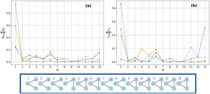
Normalized triadic occurrences (a) and fluxes (b): the aggregated network (blue color) presents a high occurrence of subgraphs \(m=1\) and \(m=13\), representing open-Vs and completely reciprocated triads, respectively. The latter covers most of the total amount of money traded. The cereals commodity layer (green color), with a high occurrence of subgraph \(m=1\). A relatively high amount of money is distributed across \(m=1\), \(m=4\) and \(m=6\). Gas/hot water/city heating layer (orange color) with a predominant occurrence and flux in subgraph \(m=1\). Agricultural services layer (pink color), with a highly heterogenous spectrum of occurrences and fluxes. Completely cyclical triads have a high occurrence in the aggregated network, but break apart when passing to single commodity layers as G.H.C and cereals, if not for rare cases such as agricultural services. In single commodity layers \(m=1\) receives the highest concentration of money, signalling a large amount of money flows over structures that greatly depend on a limited number of suppliers, which control the market..
Binary motif analysis
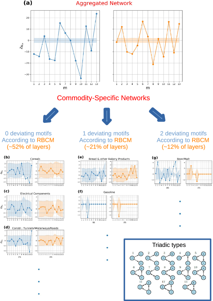
Triadic binary motif analysis: DBCM (blue circle) vs RBCM (orange circle). (a) Analysis of the aggregated network with a single representative commodity. Numerous motifs and anti-motifs are present using DBCM and RBCM as null models. (b,d) Commodity groups where RBCM reproduces all the triadic structures, and they are, respectively, cereals, electrical components, and the construction of tunnels, waterways, and roads. (e,f) Commodity groups with one network motif, namely bread and gasoline. (g) Commodity group with two network motifs, namely beer/malt. The CIs are computed by extracting the 2.5-th and 97.5-th percentile from an ensemble distribution of 500 graphs. The numerous motifs and anti-motifs in the aggregated network can be seen as the aggregation of commodity groups presenting very few characteristic patterns.
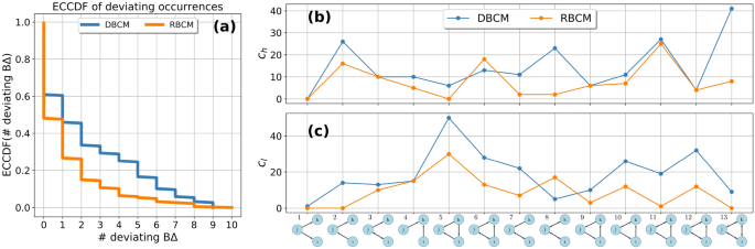
Comparison DBCM (blue circle) vs. RBCM (orange circle): (a) empirical counter cumulative distribution function ECCDF of the number of deviating binary triadic motifs and anti-motifs across commodity layers. (b) Number of commodities \(c_{h}(m)\) having a m-type motif (overoccurrence). (c) Number of commodities \(c_{l}(m)\) having a m-type anti-motif (underoccurrence). RBCM explains more triadic structures than DBCM, as shown in the difference of their ECCDF. Passing from DBCM to RBCM reduces the number of m motifs across commodities, with the exception of \(m=6\), and anti-motifs, with the exception of \(m=8\). The deviation of those triads is, hence, due to three-node correlations that go beyond directional and reciprocal tendencies of supply/use among industries. RBCM, hence, signals an increased vulnerability to demand shocks originating from the bankrupcty of industries of type k in sub-types \(m=6\) and an increased resiliency to supply/demand shocks of industries of type j in triadic formations \(m=8\)..
We analyze the number of occurrences \(N_{m}\) of all the possible triadic connected subgraphs, depicted in Fig. 1b. To quantify their deviations to randomized expectations, we define the binary z-score of subgraph m
$$\begin{aligned} z\left[ N_{m}\right] = \dfrac{N_{m}(A^*)-\langle N_{m}\rangle }{\sigma \left[ N_{m}\right] } \end{aligned}$$
(3)
where \(N_{m}(A^*)\) is the number of occurrences of the m-type subgraph in the empirical adjacency matrix, \(\langle N_{m} \rangle\) is its model-induced expected number of occurrences, and \(\sigma \left[ N_{m}\right]\) is the model-induced standard deviation.
An analytical procedure77 has been developed to compute the binary z-scores for the binary case. However, the assumption on the confidence intervals—represented as the interval \((-3,3)\)—holds true only if the ensemble distribution of \(N_{m}\) is Normal for each m. For all the commodities, m-types, and binary null models, we test the assumption using a Shapiro Test79. According to the test, \(N_{m}\) ensemble distributions are in a large proportion not normal at the \(5\%\) confidence level. Consequently, we must use a numeric approach. Networks are sampled according to the DBCM recipe by (1) computing the induced connection probability \(p_{ij; DBCM}\) and (2) establishing a link between industry i and j if and only if a uniformly distributed random number \(u_{ij} \in U(0,1)\) is below \(p_{ij; DBCM}\). The analogous recipe for RBCM requires (1) computing the set of connection probabilities for non-reciprocated connection between i and j, namely \(p_{ij}^{\rightarrow}\), \(p_{ij}^{\leftarrow}\) and \(p_{ij}^{\not \leftrightarrow}\), and reciprocated connection \(p_{ij}^{\leftrightarrow}\), generate a uniform random variable \(u_{ij} \in (0,1)\) and (2) establishing the appropriate links in the dyad in the following way:
-
a non-reciprocated link from i to j if \(u_{ij} \le p_{ij}^{\rightarrow }\);
-
a non-reciprocated link from j to i if \(u_{ij} \in (p_{ij}^{\rightarrow },p_{ij}^{\rightarrow }+p_{ij}^{\leftarrow }]\);
-
a reciprocated link from i to j (and from j to i) if \(u_{ij} \in (p_{ij}^{\rightarrow }+p_{ij}^{\leftarrow },p_{ij}^{\rightarrow }+p_{ij}^{\leftarrow }+p_{ij}^{\leftrightarrow }]\);
-
no links from i to j and from j to i otherwise.
In both cases, we generate a realization of A and extract the \(N_{m}\) statistic. \(\langle N_{m} \rangle\) and \(\sigma \left[ N_{m}\right]\), are the average and standard deviation of \(N_{m}\) extracted from the ensemble distribution of 500 realizations of A. After having computed \(z\left[ N_{m}\right]\), we also extract the 2.5-th and 97-th percentiles from the ensemble distribution of \(N_{m}\) over all models and we standardize them using Eq. (3) by replacing the empirical \(N_{m}\) with the percentile. Such measures will serve as the \(95\%\) CI for the z-score.
The results for the aggregated inter-industry network are in Fig. 3a. The z-scores computed with respect to the DBCM are depicted in blue on the left panel, while the z-scores computed with respect to the RBCM are depicted in orange on the right panel. The corresponding confidence intervals at the \(5\%\) percent are depicted with the same color (blue or orange) but in slight transparency. The majority of \(N_{m}\) are not reproduced by the randomized methods, i.e. the z-scores are outside the confidence intervals. Specifically, only \(N_{8}\) is reproduced by the DBCM, while both \(N_{1}\) and \(N_{9}\) are reproduced by the RBCM. Discounting reciprocal information does not only increase the number of triads that are statistically well described, but potentially changes their type, implying a qualitatively different z-score profile. At the same time, in the aggregated picture, \(m=1\) and \(m=9\) are seen as described by a null model implementing reciprocity, i.e. neither high dependency on suppliers (\(m=1\)), nor unstable feedback loops (\(m=9\)), where industries supply to each other in a cyclical fashion, are revealed. The aggregated network, is hence, characterized by a multitude of structures that are not well described by the null model and are due to additional three-node correlations but is relatively resilient to supply shocks and cyclical input/output. By disaggregating from the aggregated monolayer to the multi-commodity network, the majority of commodity-layers have triadic structures which are statistically reproduced by the reciprocal null model. Only 1 or 2 motifs or anti-motifs are present for the majority of the remaining commodities, a result indicating that beneath the aggregated picture, commodity groups are characterized by a small number of commodity-specific motifs and anti-motifs.
In Fig. 3b–d, z-score profiles for three commodity layers are displayed, namely cereals, electrical components, and the construction of tunnels, waterways, and roads. RBCM well describes all subgraph occurrences (\(z_{N_{m}}\) is within CI), while the DBCM signals the presence of anti-motifs for \(m=10\), \(m=11\) and \(m=12\) for cereals, and anti-motif \(m=12\) and motif \(m=13\) for the construction layer. In Fig. 3e,f, two z-score profiles are displayed—namely for bread and other bakery products and gasoline—for which RBCM signals the presence of at least a motif or anti-motif. A motif \(m=12\) is present for the former layer while an anti-motif for \(m=4\) is present for the latter. Notice that for bread the DBCM does not signal any motif or anti-motif, implying that deviations can emerge by introducing information on the reciprocal structure. Moreover, subgraph \(m=9\) in bread and the majority of subgraphs in the gasoline commodity layer are characterized by a degenerate confidence interval: in all of the generated synthetic networks \(N_{m=9}\) correspond to the empirical \(N_{9}^*\) with null variance, i.e. the constraints imposed on the ensemble totally describe the specific m-type motif, a matter which can arise regardless of the lack of statistics in the related \(N_{m}\). Finally, in Fig. 3g, the z-profile for the commodity layer beer/malt is considered. The DBCM signals a large number of motifs, specifically for \(m=2\), \(m=10\), and \(m=11\), and anti-motifs for \(m=3\) and \(m=8\). In contrast, the RBCM signals a lone motif \(m=3\) and an anti-motif \(m=6\).
In Fig. 4a, the empirical counter cumulative distribution for the number of deviating binary triads is shown. Introducing reciprocal structure information reduces the number of motifs and anti-motifs present across commodities. For instance, the percentage of commodities with at least a motif or anti-motif is \(61\%\) when compared to the DBCM, and \(48\%\) when compared to the RBCM, while the percentage of commodities having at least two motifs or anti-motifs is \(46\%\) when compared to the DBCM and \(27\%\) when compared to the RBCM.
Lastly, we identify the occurrence of m-type of motifs and anti-motifs across commodities by introducing two quantities, \(c_{h}(m)\) and \(c_{l}(m)\). \(c_{h}(m)\) represents the number of commodities having a motif of type m while \(c_{l}(m)\) represents the same measure for anti-motifs. The addition of the reciprocal structure reduces the number of commodity-specific motifs for each subgraph type, with the exception of motif \(m=6\) as depicted in Fig. 4b, and the number of anti-motifs for each type, with the exception of anti-motif \(m=8\) as depicted in Fig. 4c. The reciprocal null model, hence, reveals a higher number of commodities that are relatively more vulnerable to demand shock due to bankruptcy of industries of type k in triadic formations \(m=6\), while it reveals an increased resilience to supply/demand shocks originating from bankruptcy of industries of type j in formations \(m=8\).
Weighted motif analysis
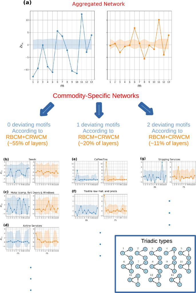
Triadic weighted motif analysis: DBCM+CReM\(_{A}\) (blue circle) vs RBCM+CRWCM (orange circle). (a) Analysis of the aggregated network with a single representative commodity. A large number of motifs and anti-motifs are present when using DBCM+CReM\(_{A}\), while three motifs are present when using the RBCM+CRWCM. (b–d) Commodity groups where RBCM+CRWCM reproduces all the triadic structures, and they are, respectively, seeds, metal components for doors and windows, and airline services. (e,f) Commodity groups with one network motif, namely Coffee/tea and textile raw materials and products. (g) Commodity group with two network motifs, namely shipping services. The CIs are computed by extracting the 2.5-th and 97.5-th percentile from an ensemble distribution of 500 graphs. Passing from the aggregated network to the disaggregated product layers unveils the presence of a few commodity-specific motifs and anti-motifs.
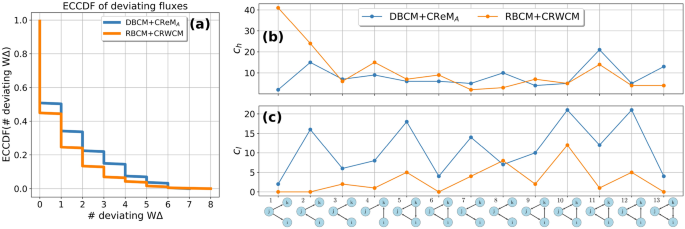
Comparison DBCM+CReM\(_{A}\) (blue circle) vs. RBCM+CRWCM (orange circle): (a) empirical counter cumulative distribution function ECCDF of the number of deviating binary triadic motifs and anti-motifs across commodity layers. (b) The number of commodities \(c_{h}(m)\) having a m-type motif. (c) The number of commodities \(c_{l}(m)\) having a m-type anti-motif. RBCM+CRWCM explains slightly more triadic fluxes than DBCM+CReM\(_{A}\), as shown in the difference of their ECCDF. Passing from the directed to the reciprocal model reduces the number of anti-motifs, with the exception of \(m=8\). In contrast, it changes qualitatively the motif profile, with a slight dominance of \(m=11\)-type motifs when the directed model is used and a clear dominance of \(m=1\)-type motifs when the reciprocal model is used. The reciprocated model unveils a vulnerability to supply shocks originating from a decrease in supply volumes of industries of type j in formations \(m=1\).
While the bankruptcy of an entire industry is unrealistic, a shock due to a decrease in the flow of goods among industries can propagate along the supply chain, with side effects on the real economy. This implies that not only binary information is important for shock propagation but also weighted information, namely the amount of money circulating on connected structures.
Consider the triadic flux \(F_{m}\) on motif m, defined as the total money circulating on triadic subgraphs of type m. We characterize the deviation of empirical \(F_{m}\) to null models by defining the weighted z-scores as
$$\begin{aligned} z\left[ F_{m}\right] = \dfrac{F_{m}(W^*)-\langle F_{m}\rangle }{\sigma \left[ F_{m}\right] } \end{aligned}$$
(4)
where \(\langle F_{m} \rangle\) is the model-induced average amount of money circulating on motif m and \(\sigma \left[ F_{m}\right]\) represents the model-induced standard deviation over the ensemble of network realizations.
The theoretical benchmark (or null model) is built by using a combination of binary and conditional weighted models, depending on the wanted constraints. If we deem reciprocal information of negligible importance we should use the combination of models given by DBCM, for the sampling of the binary adjacency matrix, and the CReM\(_{A}\), constraining the out-strength and in-strength sequences. If we deem reciprocal information necessary, a combination of the RBCM and CRWCM should be used. We compare here the two to establish the importance of the addition of reciprocity information for the detection of weighted motifs.
In operative terms, using a two-step model such as the DBCM+CReM\(_{A}\) reduces to (1) establishing a link between industries i and j when a uniform random number \(u_{ij} \in U(0,1)\) is such that \(u_{ij} \le p_{ij; DBCM}\), (2) if i and j are connected, sampling \(w_{ij}\) by using the inverse transform sampling method technique, i.e., we generate a uniformly distributed random variable \(\eta _{ij} \in U(0,1)\) such that
$$\begin{aligned} F(v_{ij})=\int _0^{v_{ij}}q_{CReM_{A}}(w_{ij}|a_{ij}=1)dw_{ij} = \eta _{ij}, \end{aligned}$$
(5)
then we invert the relationship finding the weight \(v_{ij}\) to load on the link (i, j).
The network sampling for the RBCM+CRWCM follows the same concepts with two major differences: (1) a link is established using the RBCM recipe and (2) the dyadic conditional weight probability \(q_{CReM_{A}}(w_{ij}|a_{ij}=1)\) is substituted with \(q_{CRWCM}(w_{ij}|a_{ij}=1)\) in the inverse transform sampling.
In Fig. 5a, the z-score profile for the aggregated network with a single representative commodity is depicted using the directed (in blue on the left panel) or the reciprocal models (in orange on the right panel). There is a large number of motifs and anti-motifs when the benchmark model is directed, only \(F_{3}\) does not deviate significantly.
When reciprocity information is considered, the picture changes: only three motifs, namely \(m=6\), \(m=11\), and \(m=13\), are identified, and four anti-motifs, namely \(m=3\), \(m=8\), \(m=10\), and \(m=12\), are found when the reciprocal null model is employed. This model’s enhanced accuracy unveils a higher-than-expected volume of financial activity on sub-types characterized by a single exclusive user and two suppliers utilizing each other’s products (\(m=6\)), two users supplying to each other while employing a product from the same supplier (\(m=11\)), and entirely cyclical triads (\(m=13\)). In contrast, a lower-than-expected level of financial activity transpires in open triads with two reciprocated ties (\(m=8\)), one reciprocated link and one exclusive user (\(m=3\)), or in closed triads of type \(m=10\) and \(m=12\). While it might be contended that the heightened concentration of funds on \(m=13\) is attributable to aggregation bias, it is crucial to recognize that aggregation solely accounts for the increased monetary worth of the particular sub-type in absolute terms, not for the weighted motif obtained after adjusting for the statistical null model. It should be noticed that the emergence of these specific motifs cannot be easily explained without delving into greater detail, given the representative commodity scheme, while the picture cannot be merely reduced to a higher activity on open triads and a lower activity on closed triads.
Similarly to the binary case, passing from the aggregated network to the disaggregated product-level layers, it is possible to identify a small number of commodity-specific weighted motifs and anti-motifs.
In Fig. 5b–d, three commodity layers are depicted for which no motifs and anti-motifs are present when z-scores are computed using the reciprocal model. They are ‘seeds’, ‘metal components for doors and windows’ and ‘airline services’. In the ‘seeds’ layer, the directed model signals the presence of an anti-motif for \(m=5\). In the second layer, no deviations are registered by both null models but CIs are of different nature, in fact, the reciprocal model allows a more restricted range of z-scores with respect to the directed model for \(m=9\). In the ‘airline services’ layer, for both models, no deviations are present and three CIs are degenerate for \(m=5\), \(m=9\), and \(m=10\). In Fig. 5e,f, the z-scores relative to the commodity groups ‘coffee/tea’ and ‘textile raw materials and products’ are depicted, for which 1 motif is present by using the reciprocal model. For both the directed and reciprocal models there is a weighted motif \(m=2\) in the ‘coffee/tea’ layer. In contrast, in the textile products layer the directed model signals an anti-motif for \(m=2\), while the reciprocal model signals a motif for \(m=1\). If Fig. 5g, the z-score profile for the commodity layer ‘shipping services’ is shown: the directed model signals a large number of anti-motifs, specifically for \(m=5\), \(m=7\) and \(m=12\), while it registers a motif for \(m=11\). The reciprocal model, instead, registers a motif for \(m=4\) and anti-motifs for \(m=5\) and \(m=12\). Different commodity layers call for different motifs and anti-motifs which are due to their specific characteristics. In this paper, we refrain from characterizing every single commodity layer, but a specific and thorough analysis is possible by visualizing the number of triadic sub-types, the z-score profile for \(N_{m}\) and their weighted analogs.
The empirical counter cumulative distribution ECCDF(\(\#\) deviating W\(\Delta )\) for the number of deviating weighted triads is depicted in Fig. 6a. The number of deviating triadic fluxes is steadily lower using the reciprocal model. \(F_{m}\) are maximally random for \(49\%\) when the directed model benchmark is used and for \(55\%\) according to the reciprocal model. The reduction of the number of motifs is however not as significant as in the binary case.
In Fig. 6b,c, we plot the weighted analogous of \(c_{h}(m)\) and \(c_{l}(m)\). Reciprocal information decreases the occurrence of all types of anti-motifs across commodities, with the exception of \(m=8\). Instead, the profile induced by \(c_{h}(m)\) is significantly different using the two null models. For instance, according to the directed model, \(F_{1}\) is almost always well predicted, instead, it is the most occurring motif according to the reciprocal model. At the same time, reciprocity unveils the dependency of more than 40 commodity layers on the supply of a limited amount of suppliers, which in this case control the market. In fact, the high presence of \(m=1\) weighted motif signals the vulnerability of the industry-industry network to supply shocks provoked by a reduction of supply volumes.


